'Value at
risk' (VAR or sometimes VaR) has been called the "new science of
risk management", but you do not need to be a scientist to use VAR.
Here, in part 1 of this series, we look at the idea behind VAR and
the three basic methods of calculating it. In part
2, we apply these methods to calculating VAR for a single stock
or investment.
The
Idea behind VAR
The most popular and traditional measure
of risk is volatility.
The main problem with volatility, however, is that it does not care
about the direction of an investment's movement: a stock can be
volatile because it suddenly jumps higher. (See The
Limits and Uses of Volatility.) But investors are not
distressed by gains!
For investors, risk is about the odds
of losing money, and VAR is based on that common-sense fact. By
assuming investors care about the odds of a really big loss, VAR
answers the question, "What is my worst-case scenario?" or "How much
could I lose in a really bad month?"
Now let's get specific.
A VAR statistic has three components: a time period, a confidence
level and a loss amount (or loss percentage). Keep these three parts
in mind as we give some examples of variations of the question that
VAR answers:
- What is the most I can - with a 95% or 99% level of confidence
- expect to lose in dollars over the next month?
- What is the maximum percentage I can - with 95% or 99%
confidence - expect to lose over the next year?
You can see
how the "VAR question" has three elements: a relatively high level
of confidence (typically either 95% or 99%), a time period (a day, a
month or a year) and an estimate of investment loss (expressed
either in dollar or percentage terms).
Methods of
Calculating VAR
Institutional investors use VAR to
evaluate portfolio risk, but in this introduction we will use it to
evaluate the risk of a single index that
trades like a stock: the Nasdaq 100 Index, which trades under the
ticker QQQ. The QQQ is a very
popular index of the largest non-financial stocks that trade on the
Nasdaq exchange.
There are three methods of calculating VAR:
the historical method, the variance-covariance method and the Monte
Carlo simulation.
1. Historical
Method
The historical method simply re-organizes actual
historical returns, putting them in order from worst to best. It
then assumes that history will repeat itself, from a risk
perspective.
The QQQ started trading in Mar 1999, and if we
calculate each daily return, we produce a rich data set of almost
1,400 points. Let's put them in a histogram that compares the
frequency of return "buckets". For example, at the highest point of
the histogram (the highest bar), there were more than 250 days when
the daily return was between 0% and 1%. At the far right, you can
barely see a tiny bar at 13%; it represents the one single day (in
Jan 2000) within a period of five-plus years when the daily return
for the QQQ was a stunning 12.4%!
Notice the red bars that compose the "left tail" of
the histogram. These are the lowest 5% of daily returns (since the
returns are ordered from left to right, the worst are always the
"left tail"). The red bars run from daily losses of 4% to 8%.
Because these are the worst 5% of all daily returns, we can say with
95% confidence that the worst daily loss will not exceed 4%. Put
another way, we expect with 95% confidence that our gain will exceed
4%. That is VAR in a nutshell. Let's re-phrase the statistic into
both percentage and dollar terms:
- With 95% confidence, we expect that our worst daily loss will
not exceed 4%.
- If we invest $100, we are 95% confident that our worst daily
loss will not exceed $4 ($100 x -4%).
You can see that VAR
indeed allows for an outcome that is worse than a return of -4%. It
does not express absolute certainty but instead makes a
probabilistic estimate. If we want to increase our confidence, we
need only to "move to the left" on the same histogram, to where the
first two red bars, at -8% and -7% represent the worst 1% of daily
returns:
- With 99% confidence, we expect that the worst daily loss will
not exceed 7%.
- Or, if we invest $100, we are 99% confident that our worst
daily loss will not exceed $7.
2. The
Variance-Covariance Method
This method assumes that
stock returns are normally distributed. In other words, it requires
that we estimate only two factors - an expected
(or average) return and a standard
deviation - which allow us to plot a normal distribution
curve. Here we plot the normal curve against the same actual return
data:
The idea behind the variance-covariance is similar to
the ideas behind the historical method - except that we use the
familiar curve instead of actual data. The advantage of the normal
curve is that we automatically know where the worst 5% and 1% lie on
the curve. They are a function of our desired confidence and the
standard deviation ( ): ):
The blue curve above is based on the actual daily
standard deviation of the QQQ, which is 2.64%. The average daily
return happened to be fairly close to zero, so we will assume an
average return of zero for illustrative purposes. Here are the
results of plugging the actual standard deviation into the formulas
above:
 |
3. Monte Carlo Simulation
The
third method involves developing a model for future stock price
returns and running multiple hypothetical trials through the model.
A Monte Carlo simulation refers to any method that randomly
generates trials, but by itself does not tell us anything about the
underlying methodology.
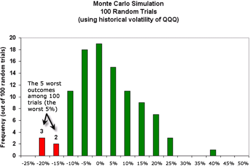
For
most users, a Monte Carlo simulation amounts to a "black box"
generator of random outcomes. Without going into further details, we
ran a Monte Carlo simulation on the QQQ based on its historical
trading pattern. In our simulation, 100 trials were conducted. If we
ran it again, we would get a different result--although it is highly
likely that the differences would be narrow. Here is the result
arranged into a histogram (please note that while the previous
graphs have shown daily returns, this graph displays monthly
returns):
 |
To summarize, we ran 100 hypothetical trials of
monthly returns for the QQQ. Among them, two outcomes were between
-15% and -20%; and three were between -20% and 25%. That means the
worst five outcomes (that is, the worst 5%) were less than -15%. The
Monte Carlo simulation therefore leads to the following VAR-type
conclusion: with 95% confidence, we do not expect to lose more than
15% during any given month.
Summary
Value at Risk (VAR) calculates
the maximum loss expected (or worst case scenario) on an investment,
over a given time period and given a specified degree of confidence.
We looked at three methods commonly used to calculate VAR. But keep
in mind that two of our methods calculated a daily VAR and the third
method calculated monthly VAR. In part 2 of this series we show you how
to compare these different time
horizons.
|


